Part 3 is here! Dive into the Weekly Tech Blog Series focused on Innovation and Cost Efficiency. If you missed it, be sure to catch the first part of the series here. Stay tuned for more insights every week!

At ShareChat, we embarked on a major redesign of the ranking system for ShareChat Feed in 2023, where we introduced a much larger and more complex Multi-gate Mixture-of-experts (MMoE) style architecture [ https://sharechat.com/blogs/artificial-intelligence/scaling-recommender-system-training-on-low-cost-gpus-at-sharechat ]. The new ranking system resulted in significant increases in retention and time spent on the platform.

However, the new ranking system came with more features, more training data, more candidates to rank, more parameters; and thus higher storage, compute, and memory requirements. This prompted us to set up a workstream to address these costs.

One of the biggest costs was the costs of inferencing the ranking model in production. In this article, we’ll focus on the work we did to reduce these costs by making inference (model serving) more efficient.

We started with very basic, low hanging fruit: making sure we run on the right kind of machines, making autoscaling work better, and then moved on to more complex changes. Overall we were able to reduce inference costs by  approximately 50% last year, and have work planned for further improvements.

Background

Before diving into the work we did, let’s briefly set some context.

ShareChat, like most social media platforms relies heavily on machine learning powered recommender systems for deciding what content and ads to show to users on our feeds.

The problem our system tries to solve can be described as follows: given all the content on the platform, which pieces of content should we show to a particular user who arrives on our app at a particular time?

We want to recommend the most relevant content for the user, using everything we know about both the user and about the content on the platform.

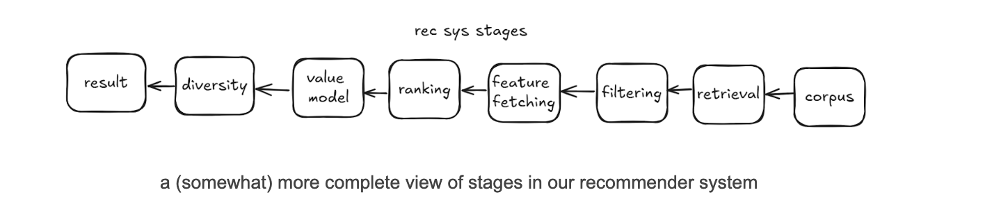
Typical recommender systems designs are composed of multiple stages. To simplify things, we can think of the system as having two stages:

• A retrieval stage, that selects between a few hundred to a few thousand candidates that are relevant for the user from a large corpus of millions. By candidates we mean posts created on the platform by our users.
• A ranking stage, that scores each candidate returned by the retrieval stage using a rich set of features that describe 1/ the user being served, 2/ the candidate being considered for them, and 3/ some request level context (time of day, etc.). The list of candidates is then sorted by this score and the top ranked candidates are used to construct the user’s feed.

A lot more happens in a production-grade recommender system, but for the purposes of this article this simplified design is informative enough. If you want to learn more about how most modern recommender systems work, this article by Nvidia is a great place to start.

Our work

Our focus here will be on the work we did to improve efficiency of the feed ranking model serving. Model serving and model inference are synonymous for the purposes of this article.

We started serving these new models in the easiest way possible, by using TensorFlow Serving on Kubernetes. This is probably the easiest way to make large TensorFlow models available for real-time inference without resorting to managed offerings like Vertex AI.

We started with easy, low hanging fruit, and then moved on to more complex changes.

1. Better capacity management

The place we started was to make sure we’re running on the right kind of capacity. The price/performance can vary significantly across machine types, so this can be one of the biggest and easiest ways to get cost savings.

For these changes, we just did quick calculations and a few local benchmarks and implemented the changes immediately, without bothering to get a precise cost saving number.

There were two things we did here:

• Maximise Spot usage.
  • Spot capacity is capacity on GCP that is offered at a much lower cost than regular (On-demand) capacity, but can be preempted at any time with little warning.
  • Spot capacity for compute SKUs on our cloud provider (GCP) is 60-90% cheaper than On-demand capacity of the same type.
  • We try to use as much Spot capacity as possible.
• Experiment with different machine types and choose the ones with the best price/performance ratio for our workload.
  • When doing inference on CPUs, performance can vary significantly depending on the exact processor family involved.
  • We found older Intel processors like Broadwell perform very poorly when compared to Skylake or newer. We also found that AMD processors give us a better price/performance ratio as compared to Intel.
  • As a result we mostly do inference with AMD processors.

2. Better autoscaling

The next area to focus on was to run on fewer machines. We run in a containerized environment and use Kubernetes for orchestration, and so we use the Horizontal Pod Autoscaler (HPA) to determine how many replicas are needed to serve production traffic.

We’ve configured HPA to scale up/down if the average CPU utilization of replicas in a deployment is higher/lower than a fixed target, for example 50%. A higher CPU utilization target means fewer machines needed to serve the same traffic, so we would like to keep the target as high as possible while staying within our service SLAs.

We found two improvements that allowed us to improve autoscaling and therefore increase our HPA target.

2.1. Reducing pod start time

Pod start time is the primary source of the lag between HPA adding new replicas and the replicas becoming available to serve traffic. We thought that if we could reduce pod start time, HPA would become faster at responding to increases in traffic, which could allow us to increase the HPA target without violating our SLAs.

We found it took 9 minutes on average for a pod to start after it had been assigned to a node (!). We dug around and found out why it took so long:

• ~2.5 minutes were spent pulling the docker image.
• ~6 minutes were spent loading the model, most of which was spent downloading the model from GCS.

The custom built TF Serving image we were using was several gigabytes in size because it had unnecessary dependencies. We built a smaller, leaner image using Docker multi-stage builds that was less than 200MB, which reduced time to pull the image to less than a minute.

Downloading the model from GCS took time because the bucket was located in the US, while model serving was done in Mumbai. We moved to a Asia based bucket which cut loading time to less than 2 minutes.

Pod start time after these changes went down to around 3 minutes.

2.2. Improving load distribution

When we took a look at CPU utilization for each instance of our service, we noticed that there was a huge difference between instances. Some were running at 30% higher utilization than others!

This is why in load tests we would notice acceptable performance at quite high utilisations, but in production we had to maintain a very low HPA target to avoid violation of our SLAs. Since HPA targets the average utilization, if some of our machines run at 40% utilization and others at 80%, you’re going to have to set the HPA target fairly low to avoid overwhelming the machines running at 80%.

If we could even out the utilization between instances, perhaps we could increase our HPA target without violating our SLAs?

The reason for the uneven utilization became clear soon: We have several machine types present in the same deployment serving production traffic. Some machine types are more powerful than others, and can serve more requests/second with the same amount of resources.  But our load balancer sent the same amount of traffic to every machine, even though we were using a smart load balancing algorithm (Least Request) that should have been loading machines based on how much they could handle.

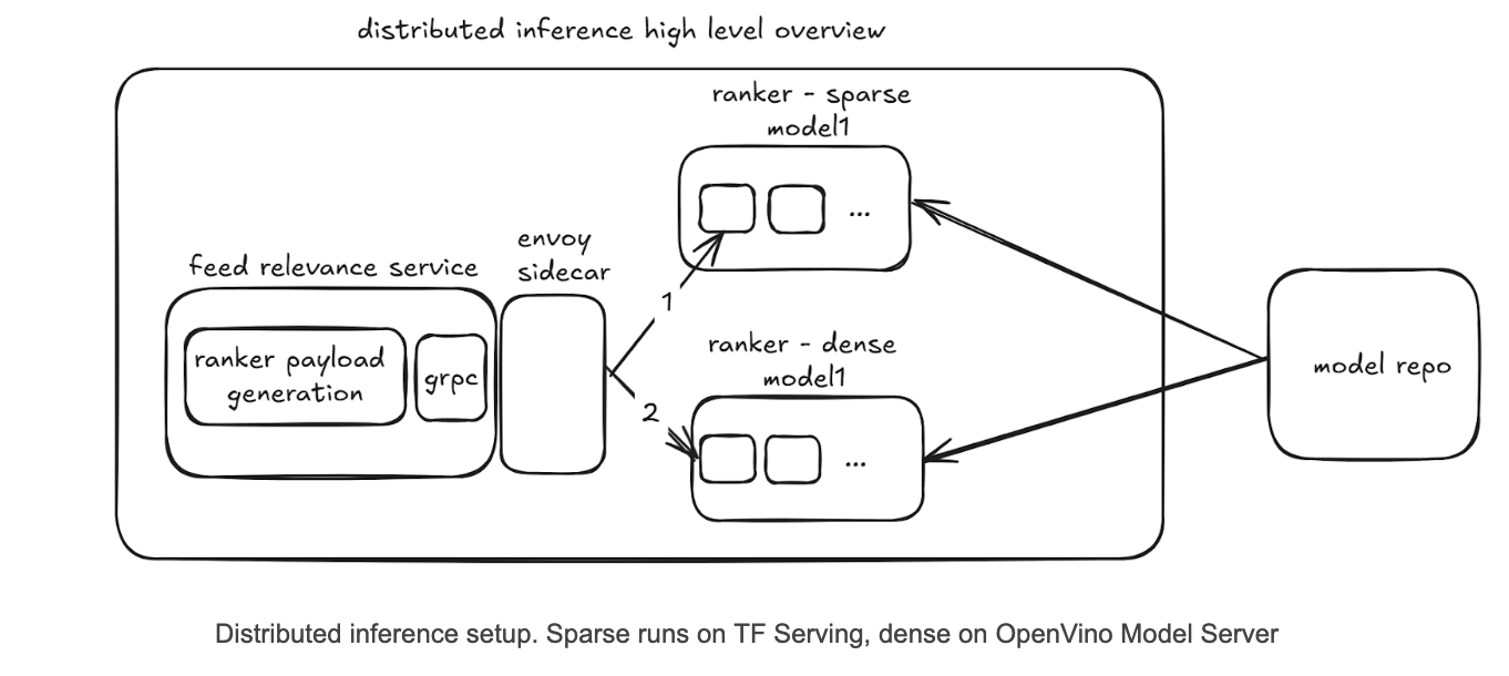
Why was least request load balancing not working as intended? We use client-side load balancing, where a downstream service called Feed Relevance Service has an Envoy sidecar that decides which model serving instance to route traffic to.

Because each Envoy sidecar only looks at its own lists of active requests to decide which model serving instance to route requests to, if you have 100s of Feed Relevance Service instances each running an Envoy sidecar, each sidecar doesn't know about active requests from the other sidecars. This leads to effectively random load balancing instead of least request.

We fixed the problem by adopting Weighted Least Request load balancing, with a separate weight for each machine type. This allows us to send more traffic to more powerful machines, making sure all machines have roughly the same CPU utilization.

After the changes to reduce pod start time and improve load distribution, we were able to increase our HPA target significantly, leading to a reduction in serving costs of 18%.

3. Using half-precision embeddings

Our model depends heavily on representations learned during training for various entity types on our platform like users, creators, and posts. The model learns a vector for each entity and stores a mapping from the entity ID (e.g., user ID) to the vector in a lookup table. These vectors are called embeddings, and the lookup table is called an embedding table.

During inference, the entity ID is provided as an input to the model, and the model uses the embedding table to convert the ID to an embedding vector. The vector can then be fed into the subsequent layers in the model just like any other numerical feature.

Because recommender systems can have very large numbers of certain kinds of entities like users and posts, embedding tables can become enormous [https://sharechat.com/blogs/artificial-intelligence/scaling-recommender-system-training-on-low-cost-gpus-at-sharechat], and can become a bottleneck to cost-effective deployment.

We found one simple change that allowed us to cut down on the memory used by our embedding tables.

We used to store embeddings in full precision (FP32). For small embedding tables this is fine, but for features like user and post IDs the embedding tables can end up being very large because of this.

For these large embedding tables, we tried using the half-precision (FP16, i.e., 16 bit floating point number) format. Half-precision trades off granularity and range of the data we can represent for lower memory usage. Interestingly, we found basically no impact to model performance at all. The impact to our offline metrics from moving to half-precision was so negligible that we didn’t even have to run an A/B test!

Moving to half-precision reduced memory usage by 35%, knocking a few percentage points off our total serving cost. This also allowed us to use lower memory VMs, giving us access to a larger pool of capacity.

4. Adopting distributed inference with OpenVino

As with most deep learning models, matrix multiplications were the most expensive operation during inference of our model. We looked into a few ways to optimize them, from tweaking the model architecture, to quantizing the model, to trying some custom third-party runtimes that could execute TensorFlow models.

We found it quite challenging to find something that reduced compute costs significantly without impacting model performance (as measured by product metrics like retention and timespent). Then we found OpenVino.

We found Intel’s OpenVino runtime to be much more performant than the TensorFlow runtime on both Intel and AMD machines. The workflow for converting TensorFlow models to OpenVino’s Intermediate Representation (IR) was also easy to use. If we converted our model to the OpenVino IR format, we could use OpenVino Model Server to serve our model instead of TensorFlow serving.

However, we discovered that certain operations (e.g., embedding lookups, tf.Example parsing) were not supported in OpenVino.

So we developed a simple kind of pipeline parallelism where we split the model into two parts:

• A sparse part that is served by TF Serving and contains ops like embedding lookups
• A dense part that is served by OpenVino Model Server and contains the dense layers.

We would first call the sparse model hosted on TF Serving, and then pass its output to the dense model hosted on OpenVino Model Server.

The new design with OpenVino handling the compute-intensive part led to a large reduction in the number of machines needed to serve our traffic, reducing costs by 40%.

We also believe this sort of distributed inference capability will be useful for future work as it allows us to scale the memory-intensive sparse part and compute-intensive dense part separately, and in the future maybe serve them on different kinds of hardware. For example, the dense part is very suitable for serving on GPUs if model complexity increases further, and removing all the custom ops makes it easy for us to serve on Nvidia GPUs using a framework like TensorRT.

What next?

The decrease in inference costs has opened up new opportunities. Some model / system changes we tried in 2024 increased timespent and retention on our platform, but also increased inference costs. Such changes often ended up being ROI-negative because the increase in timespent did not compensate for a large increase in inference costs.

With inference costs now less than half of what they were before, we expect many such changes to now be ROI-positive, and will consider revisiting them in 2025. An example of such a change is the increasing of the number of candidates ranked, which we expect to increase timespent by finding better candidates for the user, but should also increase inference costs. It was previously ROI-negative to increase candidates ranked, but may not be anymore given more efficient inference.

What about further cost optimizations? Our inference costs are quite modest after the work described above, and so in 2025 we don’t plan to make any further large investments here. We plan to focus on reducing the costs of generating and storing training data, and reducing the costs of training.

There are also two cost savings opportunities we might revisit if we had the bandwidth.

INT8 quantization

We tried to use OpenVino’s quantization workflow to INT8 quantize our models. This gave a 30% improvement in throughput on top of the previous improvements, however led to a major impact on model performance. We were unable to mitigate the drop in performance even after several rounds of tuning, so we stopped looking into INT8 quantization.

FP16 quantization should have a lower impact on model performance, but most Intel and AMD processors today only support acceleration of INT8 operations.

It’s worth digging further into which parts of the model specifically degrade the most due to quantization, and seeing if we can mitigate that somehow.

Running on GPUs

You might be wondering at this point: What about GPUs? GPUs have been the key enablers of deep learning models forever, so why don’t we use them?

We did many experiments with GPU-based inference, and some of our models do run on GPUs. Even the SC Ranker model has a slightly better price/performance on T4/L4 GPUs as compared to Intel/AMD CPUs.

However, the major issue for us in the region we run in (Mumbai) is that we don’t get much Spot GPU capacity, but there is usually plenty of Spot CPU capacity. When we compare On-demand GPUs against Spot CPUs, the price/performance for Spot CPUs is significantly better.

This other relevant factor is model architecture: Recommender system ranking models are usually not as deep as language or image models. Our production model at the moment has a single digit number of dense layers. In contrast, a commonly used image model like Resnet50 has 50 layers, and this is a model from 2015!

A model like Resnet50 will see much bigger benefits from running on GPUs than a model like ours. This should give some intuition for why at least for the moment, CPU inference is cheaper than GPU inference, when accounting for the availability of Spot CPU capacity. For the same reason, we also don’t benefit as much from quantization as say an LLM model might.

These are also things that can change: in the future we may find that making the model deeper or the layers wider delivers an increase in business metrics, and if so, we will see if the price/performance calculations change in favour of GPUs.

It should be noted that training is a different story from inference. Our training is on GPUs and would not be cost effective on CPUs. This is because training is usually done with larger batch sizes (in our case almost 20x larger), which makes the matrix multiplications very large, and large matrix multiplications is where GPUs really shine.

Conclusions

As a result of the work described above, we were able to realise a decrease in inference costs of approximately 50%. Given that inference for ranking models is one of the most expensive line items on the company’s cloud bill, we are quite happy with these results.

We will continue working on reducing inference costs, although we expect costs associated with training and training data generation to now be larger and thus be the area of focus for us in 2025.